Temperature Response

In this example, we will explore the temperature response of the filters on XRT. The temperature response provides important information on how XRT responds to the different temperatures of X-ray emissions.

import matplotlib.pyplot as plt
import numpy as np

import xrtpy

A filter channel is defined by its common abbreviation, which represents a specific type of filter used to modify the X-ray radiation observed. In this example, we will explore the carbon-on-polyimide filter (abbreviated as “C-poly”).

xrt_filter = "C-poly"

TemperatureResponseFundamental provides the functions and properties for calculating the temperature response.

date_time = "2023-09-22T21:59:59"
tpf = xrtpy.response.TemperatureResponseFundamental(
    xrt_filter, date_time, abundance_model="Photospheric"
)

To calculate the temperature response,we can do the following:

temperature_response = tpf.temperature_response()
print("Temperature Response:\n", temperature_response)

Temperature Response:
 [1.53960200e-32 2.40955299e-32 3.94741571e-32 6.98955798e-32
 1.33584492e-31 2.70949303e-31 5.75116275e-31 1.25296584e-30
 2.73372495e-30 5.83299503e-30 1.17093885e-29 2.19854631e-29
 3.97109251e-29 7.00811127e-29 1.21485095e-28 2.07573748e-28
 3.47115201e-28 5.63139260e-28 8.82892236e-28 1.33341349e-27
 1.93056016e-27 2.67696227e-27 3.59221890e-27 4.69580429e-27
 5.95497771e-27 7.37135098e-27 9.20284176e-27 1.18361192e-26
 1.53064420e-26 1.93997852e-26 2.40552580e-26 2.93333705e-26
 3.52225450e-26 4.15639575e-26 4.81169038e-26 5.46447892e-26
 6.08593035e-26 6.63102177e-26 7.03361781e-26 7.21681214e-26
 7.10604126e-26 6.65562004e-26 5.89450232e-26 5.00955448e-26
 4.24079195e-26 3.68943560e-26 3.32382295e-26 3.08153187e-26
 2.91684327e-26 2.79990204e-26 2.71207072e-26 2.64172103e-26
 2.58137263e-26 2.52669858e-26 2.47475968e-26 2.42446768e-26
 2.37516419e-26 2.32692953e-26 2.27995687e-26 2.23437522e-26
 2.19004771e-26] cm5 DN / (pix s)

We will now visualize the temperature response function using CHIANTI. These temperatures are of the plasma and are independent of the channel filter.

We use the log of the these temperatures, to enhance the visibility of the variations at lower temperatures.

chianti_temperature = np.log10(tpf.CHIANTI_temperature.to_value())

Differences overtime arise from an increase of the contamination layer on the CCD which blocks some of the X-rays thus reducing the effective area. For detailed information about the calculation of the XRT CCD contaminant layer thickness, you can refer to Montana State University.

Additional information is provided by Narukage et. al. (2011).

launch_datetime = "2006-09-22T23:59:59"

launch_temperature_response = xrtpy.response.TemperatureResponseFundamental(
    xrt_filter, launch_datetime, abundance_model="Photospheric"
).temperature_response()

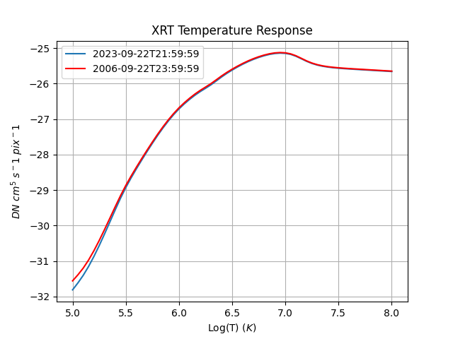
Now we can plot the temperature response versus the log of the CHIANTI temperature and compare the results for the launch date and the chosen date.

plt.figure()

plt.plot(
    chianti_temperature,
    np.log10(temperature_response.value),
    label=f"{date_time}",
)
plt.plot(
    chianti_temperature,
    np.log10(launch_temperature_response.value),
    label=f"{launch_datetime}",
    color="red",
)

plt.title("XRT Temperature Response")
plt.xlabel("Log(T) ($K$)")
plt.ylabel("$DN$ $cm^5$ $ s^-1$ $pix^-1$")
plt.legend()
plt.grid()

plt.show()