Exploring XRT’s Configuration

This example explores the X-Ray Telescope (XRT) instrument properties using XRTpy’s xrtpy.response.Channel. It provides convenient methods and attributes to access and analyze various aspects of the XRT instrument configuration.

import matplotlib.pyplot as plt

import xrtpy

We begin by defining a filter channel by its common abbreviation. In this example we will be exploring the titanium-on-polyimide filter. For detailed information about various filter channels and their characteristics, you can refer to The X-Ray Telescope.

To explore the properties and characteristics of a defined filter channel, we will create a xrtpy.response.Channel. By passing in the filter name as an input, we can work with the properties associated with the titanium-on-polyimide filter.

channel = xrtpy.response.Channel("Ti-poly")

Now that we have created our channel, we can delve into the XRT instrument and its properties. We will start by examining basic information about the XRT instrument.

print("Selected filter:", channel.name)
print("\nObservatory:", channel.observatory)
print("Instrument:", channel.instrument)

Selected filter: Ti-poly

Observatory: Hinode
Instrument: XRT

It is important to note that most instrument properties of XRT remain the same regardless of the specific filter being used. This means that many characteristics and specifications of the XRT instrument, such as its dimensions, field of view, and detector properties, are independent of the selected filter.

We can explore various characteristics of the the Charge-Coupled-Device (CCD) camera camera, such as its quantum efficiency and pixel size to list a few.

print(channel.ccd.ccd_name)
print("\nPixel size: ", channel.ccd.ccd_pixel_size)
print("Full well: ", channel.ccd.ccd_full_well)
print("Gain left: ", channel.ccd.ccd_gain_left)
print("Gain right: ", channel.ccd.ccd_gain_right)
print("eV pre electron: ", channel.ccd.ccd_energy_per_electron)

Hinode/XRT Flight Model CCD

Pixel size:  13.5 micron
Full well:  222000.0 electron
Gain left:  58.79999923706055 electron / DN
Gain right:  57.5 electron / DN
eV pre electron:  3.6500000953674316 eV / electron

We can explore the XRT entrance filter properties utilizing entrancefilter.

print(channel.entrancefilter.entrancefilter_name)
print("Material: ", channel.entrancefilter.entrancefilter_material)
print("Thickness: ", channel.entrancefilter.entrancefilter_thickness)
print("Density: ", channel.entrancefilter.entrancefilter_density)

Entrance filters
Material:  ['Al2O3' 'Al' 'Al2O3' 'polyimide']
Thickness:  [  75. 1492.    0. 2030.] Angstrom
Density:  [3.97  2.699 3.97  1.43 ] g / cm3

XRT data is recorded through nine X-ray filters, which are implemented using two filter wheels.

By utilizing the channel.filter_# notation, where # represents filter wheel 1 or 2, we can explore detailed information about the selected XRT channel filter.

It’s worth noting that sometimes the other filter will yield the result “Open,” as it’s not use. For more comprehensive information about the XRT filters, you can refer to The X-Ray Telescope.

print("Filter Wheel:", channel.filter_2.filter_name)
print("\nFilter material:", channel.filter_2.filter_material)
print("Thickness: ", channel.filter_2.filter_thickness)
print("Density: ", channel.filter_2.filter_density)

Filter Wheel: Ti filter on polyimide

Filter material: ['TiO2' 'Ti' 'TiO2' 'polyimide']
Thickness:  [  75. 2338.    0. 2522.] Angstrom
Density:  [4.26 4.54 4.26 1.43] g / cm3

We can explore geometry factors in the XRT using geometry.

print(channel.geometry.geometry_name)
print("\nFocal length:", channel.geometry.geometry_focal_len)
print("Aperture Area:", channel.geometry.geometry_aperture_area)

Hinode/XRT Flight Model geometry

Focal length: 270.753 cm
Aperture Area: 2.28 cm2

The XRT is equipped with two mirrors and We can access the properties of these mirrors using the channel_mirror_# notation, where # represents the first or second mirror surface.

print(channel.mirror_1.mirror_name)
print("Material: ", channel.mirror_1.mirror_material)
print("Density: ", channel.mirror_1.mirror_density)
print("Graze_angle: ", channel.mirror_1.mirror_graze_angle)

Hinode/XRT Flight Model mirror
Material:  Zerodur
Density:  2.5299999713897705 g / cm3
Graze_angle:  0.9100000262260437 deg

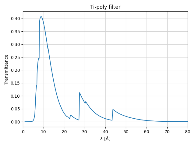
Finally we can explore the XRT transmission properties

plt.figure()

plt.plot(channel.wavelength, channel.transmission, label=f"{channel.name}")
plt.title(f"{channel.name} filter")
plt.xlabel(r"$\lambda$ [Å]")
plt.ylabel(r"Transmittance")
# The full range goes up to 400 Å, but we will limit it to 80 Å for better visualization
plt.xlim(0, 80)
plt.grid(color="lightgrey")
plt.tight_layout()

plt.show()