Using temperature_from_filter_ratio to analyze XRT data

This example demonstrates how to use temperature_from_filter_ratio to calculate the temperature and emission measure in an image using the filter ratio method.

First we need to import temperature_from_filter_ratio.

As an example we will use the test data included in XRTpy, though data with the right characteristics in the XRT archive could also be used. It’s necessary to use two images that are the same size and different filters. To get good results the images should have been taken close in time as well, ideally adjacent in time. Note that not all filter ratios produce good results.

This data was generated using the IDL routine xrt_prep.pro from SolarSoft and is unnormalized. Data in the Level 1 archive are normalized, which is also okay to use, though the IDL routine xrt_teem.pro did not allow that. For normalized data the image data is multiplied by the exposure time before analysis.

import sunpy.map
from sunpy.net import Fido
from sunpy.net import attrs as a

from xrtpy.response.temperature_from_filter_ratio import temperature_from_filter_ratio

/home/docs/checkouts/readthedocs.org/user_builds/xrtpy/envs/latest/lib/python3.11/site-packages/tqdm/auto.py:21: TqdmWarning: IProgress not found. Please update jupyter and ipywidgets. See https://ipywidgets.readthedocs.io/en/stable/user_install.html
  from .autonotebook import tqdm as notebook_tqdm

result = Fido.search(
    a.Time("2011-01-28 01:31:55", "2011-01-28 01:32:05"), a.Instrument("xrt")
)

data_files = Fido.fetch(result, progress=False)

file1 = data_files[1]
file2 = data_files[0]
print("Files used:\n", file1, "\n", file2)

Files used:
 /home/docs/sunpy/data/l1_xrt20110128_013204_9.fits
 /home/docs/sunpy/data/l1_xrt20110128_013155_9.fits

temperature_from_filter_ratio uses Sunpy maps as input.

map1 = sunpy.map.Map(file1)
map2 = sunpy.map.Map(file2)

print(
    map1.fits_header["TELESCOP"],
    map1.fits_header["INSTRUME"],
)
print(
    "\n File 1 used:\n",
    file1,
    "\n Observation date:",
    map1.fits_header["DATE_OBS"],
    map1.fits_header["TIMESYS"],
    "\n Filter Wheel 1:",
    map1.fits_header["EC_FW1_"],
    map1.fits_header["EC_FW1"],
    "\n Filter Wheel 2:",
    map1.fits_header["EC_FW2_"],
    map1.fits_header["EC_FW2"],
    "\n Dimension:",
    map1.fits_header["NAXIS1"],
    map1.fits_header["NAXIS1"],
)

print(
    "\nFile 2 used:\n",
    file2,
    "\n Observation date:",
    map2.fits_header["DATE_OBS"],
    map2.fits_header["TIMESYS"],
    "\n Filter Wheel 1:",
    map2.fits_header["EC_FW1_"],
    map2.fits_header["EC_FW1"],
    "\n Filter Wheel 2:",
    map2.fits_header["EC_FW2_"],
    map2.fits_header["EC_FW2"],
    "\n Dimension:",
    map2.fits_header["NAXIS1"],
    map2.fits_header["NAXIS1"],
)

HINODE XRT

 File 1 used:
 /home/docs/sunpy/data/l1_xrt20110128_013204_9.fits
 Observation date: 2011-01-28T01:32:04.998 UTC (TBR)
 Filter Wheel 1: Be_thin 3
 Filter Wheel 2: Open 0
 Dimension: 384 384

File 2 used:
 /home/docs/sunpy/data/l1_xrt20110128_013155_9.fits
 Observation date: 2011-01-28T01:31:55.932 UTC (TBR)
 Filter Wheel 1: Open 0
 Filter Wheel 2: Ti_poly 2
 Dimension: 384 384

The temperature_from_filter_ratio function has several options, mirroring the IDL routine xrt_teem.pro in SolarSoft in most respects. A simple call with no extra parameters calculates the temperature and (volume) emission measure for the two images without any binning or masking of the data.

T_EM = temperature_from_filter_ratio(map1, map2)
T_e = T_EM.Tmap

The output of temperature_from_filter_ratio is a namedtuple of SunPy maps with attributes Tmap, EMmap, Terrmap, and EMerrmap. As with the SolarSoft IDL routine xrt_teem.pro, the output images are logs of the quantities. Tmap.data is the electron temperature, EMmap.data is the volume emission measure, Terrmap.data is a measure of the uncertainties in the temperature determined for each pixel and EMerrmap.data is the same for the emission measure. Each map has data and associated metadata. To examine the results one can use matplotlib and sunpy:

import matplotlib.pyplot as plt
import numpy as np
from sunpy.coordinates.sun import B0, angular_radius
from sunpy.map import Map

# To avoid error messages from sunpy we add metadata to the header:
rsun_ref = 6.95700e08
hdr1 = map1.meta
rsun_obs = angular_radius(hdr1["DATE_OBS"]).value
dsun = rsun_ref / np.sin(rsun_obs * np.pi / 6.48e5)
solarb0 = B0(hdr1["DATE_OBS"]).value
hdr1["DSUN_OBS"] = dsun
hdr1["RSUN_REF"] = rsun_ref
hdr1["RSUN_OBS"] = rsun_obs
hdr1["SOLAR_B0"] = solarb0

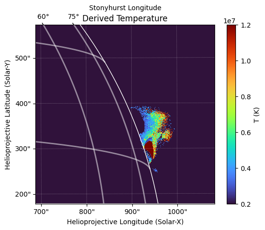
fig = plt.figure()
# We could create a plot simply by doing T_e.plot(), but here we choose to make a linear plot of T_e
m = Map((10.0**T_e.data, T_e.meta))
m.plot(title="Derived Temperature", vmin=2.0e6, vmax=1.2e7, cmap="turbo")
m.draw_limb()
m.draw_grid(linewidth=2)
cb = plt.colorbar(label="T (K)")

See the temperature_from_filter_ratio.py script for more information. Among the options are verbose output, binning the data by an integer factor (to increase the signal to noise), specifying a temperature range to examine, providing a mask for excluding regions of the images from the analysis, and setting error thresholds on the temperature and photon noise that differ from the default values.

These data were analyzed by Guidoni et al. (2015, ApJ 800, 54). See also Narukage et al. (2014, Solar Phys. 289, 1029).