Deriving temperatures using composite images and the filter ratio method

The temperature_from_filter_ratio routine in XTRpy derives the temperature and emission measure in XRT images by using two images taken at nearly the same time but using different filters. When doing this you can use standard XRT Level 1 data files or you can use “composite” images. Composite images are created from two or three images taken sequentially with the same pointing and filter but with different exposure times. Generally one wants to use either a long and short pair of exposures or a long-medium-short triple of exposures. Such composite images are made routinely for the synoptic archive of Hinode. The idea behind composite images is that pixels in the image that are saturated in the long exposure are replaced by pixels from the short (or medium) exposure that are not saturated and thus create an image with a greater dynamic range than you would get with a single image.

We start by importing temperature_from_filter_ratio.

To use composite images, we need to generate their exposure maps, which are images where each pixel value is the exposure time of the image from which the pixel came. Most of the pixels will generally be from the long exposure image, but for the brightest part of the image, the pixels will come from the medium or short exposure image that was used to generate the composite image. The composite images that we’ll use can be downloaded from the XRT archive.

For this example, we will use the download_file utility from astropy to download the composite files. We also use the routine filename2repo_path from XRTpy to find the correct URL for each file to be downloaded.

from astropy.utils.data import download_file

from xrtpy.response.temperature_from_filter_ratio import temperature_from_filter_ratio
from xrtpy.util.filename2repo_path import filename2repo_path

filename1 = "comp_XRT20210730_175810.1.fits"
filename2 = "comp_XRT20210730_175831.6.fits"
url1 = filename2repo_path(filename1, join=True)
url2 = filename2repo_path(filename2, join=True)
# These files will go under your astropy cache directory, typically ~/.astropy/cache/download/url/
file1 = download_file(url1)
file2 = download_file(url2)

/home/docs/checkouts/readthedocs.org/user_builds/xrtpy/envs/latest/lib/python3.11/site-packages/tqdm/auto.py:21: TqdmWarning: IProgress not found. Please update jupyter and ipywidgets. See https://ipywidgets.readthedocs.io/en/stable/user_install.html
  from .autonotebook import tqdm as notebook_tqdm

Then we need to calculate the exposure maps, which will be used with temperature_from_filter_ratio.

from xrtpy.util.make_exposure_map import make_exposure_map

expmap1 = make_exposure_map(file1)
expmap2 = make_exposure_map(file2)

Note that each call to this routine will result in more files being downloaded. Now we are ready to call temperature_from_filter_ratio. This routine takes Sunpy maps as input (not related to exposure maps).

from sunpy.map import Map

map1 = Map(file1)
map2 = Map(file2)
T_EM = temperature_from_filter_ratio(map1, map2, expmap1=expmap1, expmap2=expmap2)

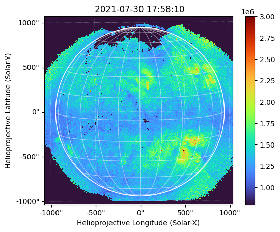
temperature_from_filter_ratio returns a named tuple of maps: Tmap, EMmap, Terrmap, EMerrmap. To make a nice looking plot, we use matplotlib.

import matplotlib.pyplot as plt

fig = plt.figure()
T_e = T_EM.Tmap
m = Map(10.0**T_e.data, T_e.meta)
m.plot(vmin=8.0e5, vmax=3.0e6, cmap="turbo")
m.draw_limb()
m.draw_grid()
cb = plt.colorbar()
plt.show()