Temperature Response Analysis for X-Ray Telescope (XRT)

This notebook explores the temperature response of X-ray channels in the X-Ray Telescope (XRT). The temperature response provides valuable insights into how the XRT instrument detects and responds to different temperatures of X-ray emissions. By assuming a specific spectral emission model at a given date, we can investigate the behavior of the XRT channels.

To begin the analysis, we will import the necessary packages that enable us to perform the temperature response calculations and generate visualizations.

import matplotlib.pyplot as plt
import numpy as np

import xrtpy

Let’s dive in and explore the fascinating temperature response characteristics of the XRT!

Contents

1. Define a Filter Channel

2. Define Date & Time

3. Temperature-Response-Fundamental

4. Temperature Response Function

5. Plot Temperature Response

Define a Filter Channel

A filter channel is defined by its common abbreviation, which represents a specific type of filter used to modify the X-ray radiation passing through. In this example, we will explore the carbon-on-polyimide filter (abbreviated as “C-poly”).

For detailed information about various filter channels and their characteristics, you can refer to the xrtpy- X-Ray Filter Channel section.

filter_ = "C-poly"

Define a date and time

In order to analyze the temperature response, it is necessary to specify a date and time for the analysis. The date and time can be defined together using specific string formats. To explore the data captured a year after the launch date, we will define the date and time accordingly.

For detailed examples and further information about date and time string formats, you can refer to the sunpy-time documentation.

date_time = "2007-09-22T21:59:59"

TemperatureResponseFundamental

The TemperatureResponseFundamental object is a crucial component that provides all the necessary functions and properties for calculating the temperature response in our analysis. By referencing this object, we can access the required methods and attributes for further calculations.

To create a TemperatureResponseFundamental object, you need to provide the defined filter channel (Filter) and the desired date and time (date_time). Additionally, you can specify the abundance model of interest, such as Photospheric, which influences the temperature response calculations.

Temperature_Response_Fundamental = xrtpy.response.TemperatureResponseFundamental(
    filter_, date_time, abundance_model="Photospheric"
)

Temperature Response function

To calculate the temperature response, simply call the temperature_response() function on the Temperature_Response_Fundamental object. This function utilizes the specified filter, date, and abundance model to generate the temperature response as a result.

temperature_response = Temperature_Response_Fundamental.temperature_response()

The temperature_response() function returns the temperature response for the selected filter, date, and time. The returned value is an astropy-quantity object with associated astropy.units.

print("Temperature Response:\n", temperature_response)

Temperature Response:
 [1.75050807e-32 2.70263514e-32 4.36848081e-32 7.64222509e-32
 1.44553318e-31 2.90457420e-31 6.10688786e-31 1.31813616e-30
 2.85199117e-30 6.04093244e-30 1.20584729e-29 2.25580103e-29
 4.06436412e-29 7.15874537e-29 1.23900438e-28 2.11433884e-28
 3.53237680e-28 5.72715150e-28 8.97569641e-28 1.35530879e-27
 1.96217565e-27 2.72120713e-27 3.65282015e-27 4.77711444e-27
 6.06054054e-27 7.50321445e-27 9.36405909e-27 1.20323078e-26
 1.55414815e-26 1.96738272e-26 2.43687806e-26 2.96895640e-26
 3.56257848e-26 4.20174413e-26 4.86211023e-26 5.51967813e-26
 6.14517852e-26 6.69301462e-26 7.09635243e-26 7.27766017e-26
 7.16208307e-26 6.70431811e-26 5.93449932e-26 5.04143353e-26
 4.26660561e-26 3.71134670e-26 3.34334665e-26 3.09955692e-26
 2.93387374e-26 2.81622487e-26 2.72785171e-26 2.65705658e-26
 2.59631790e-26 2.54128549e-26 2.48900542e-26 2.43838341e-26
 2.38875772e-26 2.34020863e-26 2.29292986e-26 2.24705072e-26
 2.20243354e-26] cm5 DN / (pix s)

Plotting the Temperature-Response

In this section, we will visualize the temperature response by plotting the temperature_response function against the corresponding temperatures. It’s important to note that the CHIANTI temperatures used in this plot are the temperatures of the solar plasma and are independent of the channel filter.

The CHIANTI temperatures are stored in the Temperature_Response_Fundamental object and are provided in units of Kelvin (K). These temperatures serve as the independent variable for plotting the temperature response.

By visualizing the temperature response, we can gain insights into how it varies with respect to temperature, providing a deeper understanding of the XRT channelcharacteristics.

Additionally, if you wish to explore more details about the CHIANTI database, you can find further information at chiantidatrbase.org.

CHIANTI_temperature = Temperature_Response_Fundamental.CHIANTI_temperature

We take the log of the CHIANTI_temperature for plotting, which compresses the scale and enhances the visibility of the variations for lower temperatures.

log_CHIANTI_temperature = np.log10(CHIANTI_temperature.value)

In addition, we will compare the data shortly after the spacecraft launch date with the current data. This allows us to identify any differences or variations in the temperature response over time.

We define a new temperature response data for the launch date. The process for obtaining this data is the same as previously shown, where we specify the filter, launch date, and abundance model.

By comparing the temperature response at the launch date with the current temperature response, we can gain insights into any changes that may have occurred over time. This comparison helps us understand the stability and evolution of the XRT.

launch_date_time = "2006-09-22T23:59:59"

launch_date_temperature_response = xrtpy.response.TemperatureResponseFundamental(
    filter_, launch_date_time, abundance_model="Photospheric"
).temperature_response()

Create a plotting function that plots the temperature_response versus log_CHIANTI_temperature for the chosen filter, date, and time.

def plotting_temperature_response():
    plt.figure(figsize=(30, 12))

    plt.plot(
        log_CHIANTI_temperature,
        np.log10(temperature_response.value),
        linewidth=4,
        label=f"{filter_} {date_time}",
    )
    plt.plot(
        log_CHIANTI_temperature,
        np.log10(launch_date_temperature_response.value),
        linewidth=3,
        label=f"{filter_} {launch_date_time}",
        color="red",
    )

    plt.title("XRT Temperature Response", fontsize=30)
    plt.xlabel("Log(T) ($K$)", fontsize=27)
    plt.ylabel("$DN$ $cm^5$ $ s^-1$ $pix^-1$", fontsize=27)
    plt.legend(fontsize=30)

    plt.xticks(fontsize=25)
    plt.yticks(fontsize=25)

    plt.grid()
    plt.show()

Run plotting_temperature_response function to create the plot.

plotting_temperature_response()

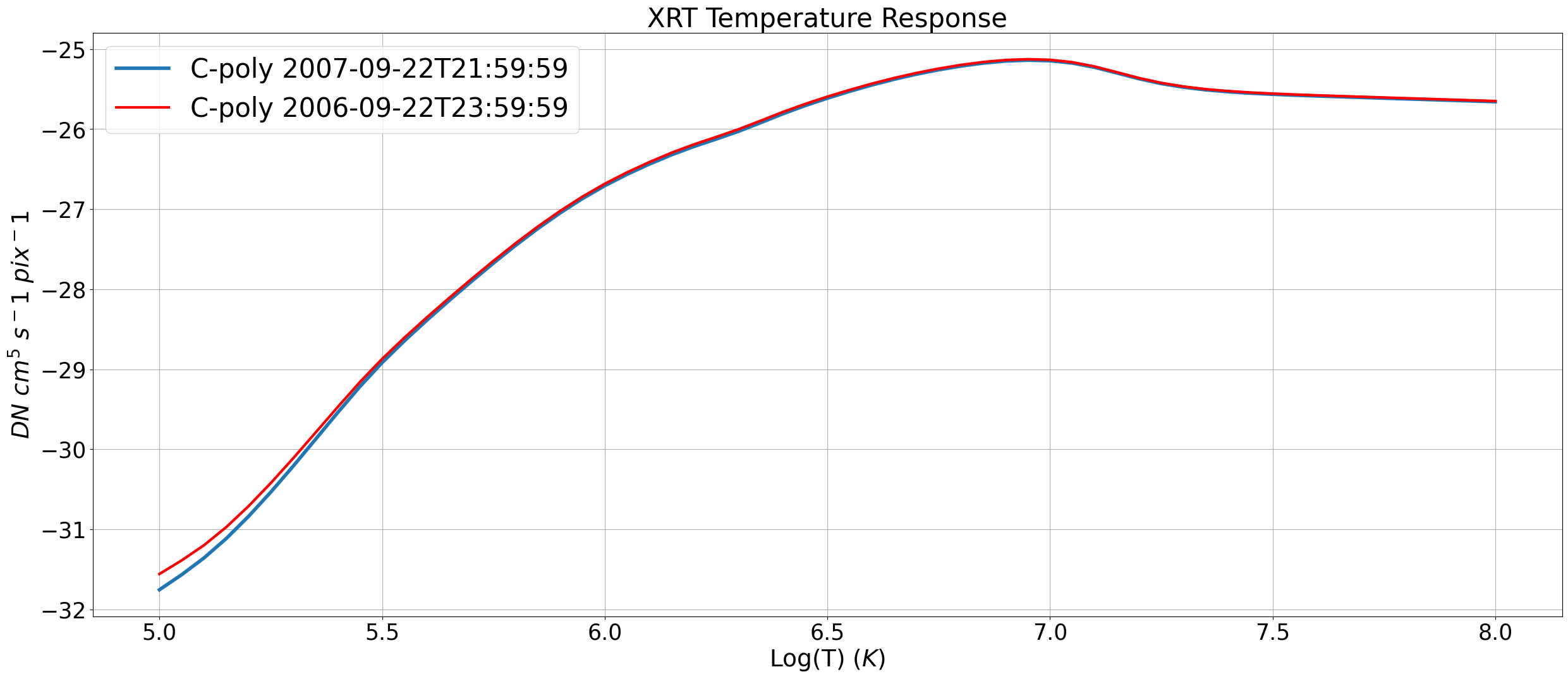
Plotting the temperature response at launch date and a year after highlights the differences. This is due to the contamination layer thickness on the CCD. Information about the XRT CCD contaminant layer thickness calculation can be found at Montana State University Solar Physics site. In addition, more information can be found referencing Narukage et. al. (2011).