Effective Area Analysis for X-Ray Telescope (XRT)

In this example, we will explore the effective areas for different XRT filter channels, considering their respective thicknesses of the CCD contamination layer at a specific date and time. Understanding the effective areas is essential for accurately interpreting and quantifying X-ray signals. Let’s dive into the details and calculations below.

# Import the xrtpy module for X-ray Telescope (XRT) calculations
import xrtpy

Contents

1. Define Filter

2. Define Date & Time

3. Effective-Area-Fundamental

4. Effective Area Function

5. Plotting the Effective Area versus Wavelength

Define a Filter Channel

In XRT analysis, the filter channels play a crucial role in determining the effective areas. A filter channel refers to a specific configuration of filter materials. By defining the filter channel appropriately, we can accurately calculate the effective area for a given XRT configuration.

Let’s begin by defining a filter channel using its abbreviation. For example, if we want to explore the effective area for an aluminum-on-polyimide filter channel, we need to specify the relevant abbreviation. This step ensures that we consider the correct filter configuration in our calculations. Refer to the xrtpy- X-Ray Filter Channel section for more information.

# Define the filter channel abbreviation
Filter = "Al-poly"

Define a date and time

Let’s consider exploring the data captured approximately a year after the launch date. We need to define a specific date and time. We will use the format “YYYY-MM-DD HH:MM:SS” to represent the desired date and time. The date and time can be specified using various formats depending on your preference and data availability. Please refer to the sunpy-time documentation for detailed examples and further information on different date and time string formats.

# Define the date and time for analysis
date_time = "2007-09-22T22:59:59"

EffectiveAreaFundamental

The EffectiveAreaFundamental object plays a central role in calculating the effective area. It provides a range of functions and properties that are essential for this computation. By utilizing the EffectiveAreaFundamental object, we can accurately determine the effective area based on the specified filter channel, date, and time.

To access the functionality of the EffectiveAreaFundamental object, we need to reference it by inserting the defined Filter and date_time.

# Create an instance of the EffectiveAreaFundamental object
Effective_Area_Fundamental = xrtpy.response.EffectiveAreaFundamental(Filter, date_time)

Effective Area function

To actually calculate the effective area function we call the effective_area() method of the Effective_Area_Fundamental object.

# Calculate the effective area
effective_area = Effective_Area_Fundamental.effective_area()

The effective_area function returns the effective area for a selected filter, date, and time as an astropy-quantity with astropy.units.

print("Effective Area:\n", effective_area)

Effective Area:
 [2.78457457e-10 7.94914547e-10 2.06647656e-09 ... 2.07749128e-15
 0.00000000e+00 0.00000000e+00] cm2

Plotting the Effective Area versus Wavelength

To gain insights into the X-ray Telescope (XRT) observations, we will plot the effective area against the corresponding wavelengths. This visualization allows us to understand how the effective area varies across different wavelengths and provides valuable information for interpreting XRT data.

We will utilize the channel_wavelength property within the Effective_Area_Fundamental object to get the wavelengths.

# Wavelength unit in Angstroms A˚
wavelength = Effective_Area_Fundamental.channel_wavelength

To further analyze the effective area data, we will focus on the observations relative to the spacecraft launch date. This will allow us to identify any differences or trends in the effective area during the early stages of the mission. We will define the effective area data for the launch date in the same manner as previously shown.

# Create an instance of the EffectiveAreaFundamental object for the launch date and time of the same filter channel
relative_launch_date_time = "2006-09-22T22:59:59"

EAF_launch_date_time = xrtpy.response.EffectiveAreaFundamental(
    Filter, relative_launch_date_time
)

# launch date effective area
launch_date_effective_area = EAF_launch_date_time.effective_area()

Create a plotting function that plots the effective area versus wavelegth.

def plot_effective_area():
    import matplotlib.pyplot as plt

    plt.figure(figsize=(30, 13))

    plt.plot(
        wavelength,
        effective_area,
        linewidth=8,
        label=f"{Filter} {date_time}",
    )

    plt.plot(
        wavelength,
        launch_date_effective_area,
        linewidth=8,
        label=f"{Filter} {relative_launch_date_time}",
    )

    plt.title("XRT Effective Area\nAl-Poly", fontsize=30)
    plt.xlabel("Wavelength (Å)", fontsize=30)
    plt.ylabel("Effective Area ($cm^{2}$)", fontsize=30)
    plt.legend(fontsize=30)

    plt.xticks(fontsize=27)
    plt.yticks(fontsize=27)
    plt.xlim(0, 60)

    plt.grid(color="lightgrey")
    plt.show()

Run plot_effective_area function to create the plot.

plot_effective_area()

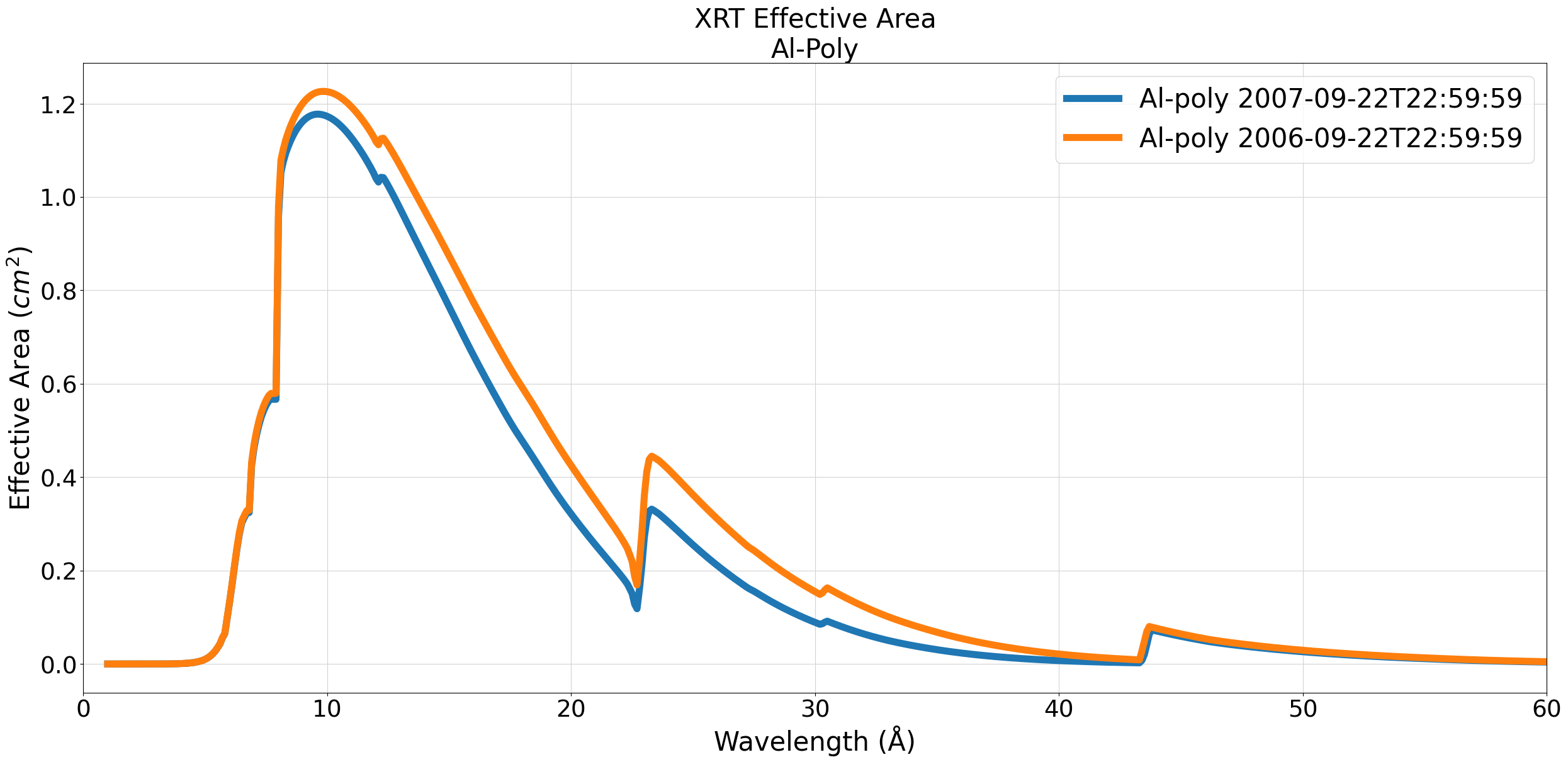
By plotting the effective area at the spacecraft launch date and comparing it to the effective area a year after, we can observe and analyze any differences. These differences arise from variations in the contamination layer thickness on the CCD which blocks some of the X-rays thus reducing the effective area. For detailed information about the calculation of the XRT CCD contaminant layer thickness, you can refer to the Montana State University Solar Physics site.

To further understand the factors contributing to the observed differences, additional information can be found in the research paper by Narukage et. al. (2011). This paper provides valuable insights into the characteristics and behavior of the XRT instrument, which can aid in interpreting the effective area data.